Introduction

To implement complex domains, we use the concept of constructive solid geometry to build SDFs from simple primiatives.

The SDFs implemented were inspired by Inigo Quilez SDFs, They have provided a wide library of 2D and 3D SDFs, and detailed comments about use.

We use the dune package here for visualization and demonstration purposes:

[1]:

import dune.grid
import numpy as np
from matplotlib import pyplot as plt
from matplotlib.collections import PatchCollection
from matplotlib.patches import Polygon, Rectangle, Wedge
from ufl import SpatialCoordinate, as_vector, pi

from ddfem.plot import plotSdfTree

gridView = dune.grid.structuredGrid([-1.1, -1.1], [1.1, 1.1], [110, 110])


def plotSDF(sdf):
    plotSdfTree(sdf, gridView, figsize=[12, 8], gridLines=None)

Shapes

[2]:

from ddfem.geometry import Arc, Box, Ball, Pie, Vesica

Arc

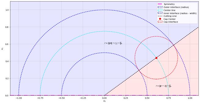
Denoting, \(p = (x_0, |x_1|)^T\), \(r_c = R - \frac{W}{2}\), \(c = r_c (\cos(\theta), \sin(\theta))^T\). We have the signed distance function for an arc centered at the origin,

\[\begin{split}r(x) = - \frac{W}{2} + \begin{cases} \| p - c \| & \text{if } p_0 \sin(\theta) > p_1 \cos(\theta) \\ \left| \|p\| - r_c \right| & \text{otherwise} \end{cases}\end{split}\]

where \(W\) is the width of the arc, \(R\) is the radius of the outer interface, and \(\theta\) is the angle of the opening.

[4]:

arcFigure()

[5]:

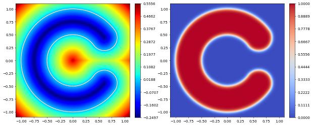
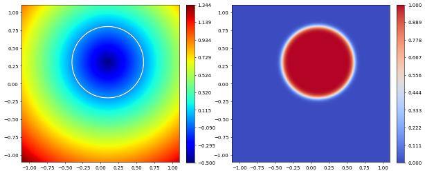
arc = Arc(radius=1, angle=0.2 * pi, width=0.5, center=(0.1, 0.3), epsilon=0.1)
plotSDF(arc)

Box

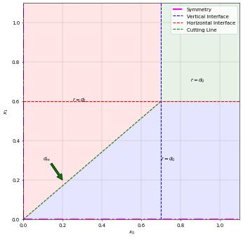
Denoting, \(d = \left( |x_0| - \frac{W}{2}, |x_1| - \frac{H}{2} \right)^T\), and \(d_m = max(d_0, d_1)\).

We have the signed distance function for a box centered at the origin,

\[\begin{split}r(x) = \begin{cases} \| \left( \max(d_0, 0), \max(d_1, 0) \right)^T \| & \text{if } d_m > 0 \\ d_m & \text{otherwise} \end{cases}\end{split}\]

where \(W\) is the width of the box, and \(H\) is the height of the box.

[7]:

boxFigure()

[8]:

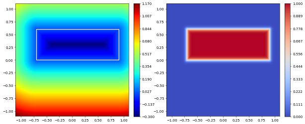
box = Box(width=1.6, height=0.6, center=(0.1, 0.3), epsilon=0.1)
plotSDF(box)

Ball

We have the signed distance function for a ball centered at the origin,

\[r(x) = |x| - R\]

where \(R\) is the radius of the Ball.

[9]:

circle = Ball(radius=0.5, center=(0.1, 0.3), epsilon=0.1)
plotSDF(circle)

Pie

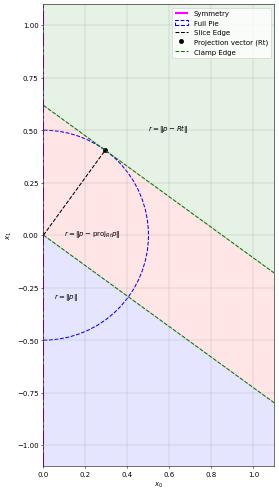
Denoting, \(p = (|x_0|, x_1)^T\), \(t = (\sin(\theta/2), \cos(\theta/2))^T\). We have the signed distance function for an pie centered at the origin,

\[r(x) = \max( \| p \| - R, \| p - \max(0, \min(R, p \cdot t)) t \| \text{sign}(p \times t) )\]

\(R\) is the radius of the full circle pie, and \(\theta\) is the angle of the slice.

Note, \(\max(0, \min(p \cdot t, R)) t\) is to project \(p\) onto \(t\), \(\text{proj}_{t}{p}\); while limiting to only on the interface edge. This gives the distance from this line. Also, to determine if the point is inside or outside the wedge, the sign of the 2D cross product is used.

[11]:

pieFigure()

[12]:

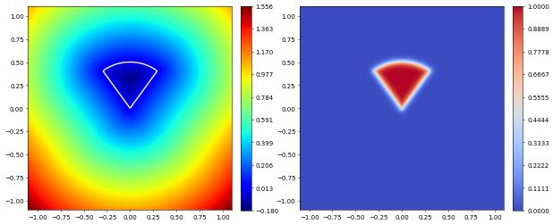
pie = Pie(radius=0.5, angle=0.4 * pi, epsilon=0.1)
plotSDF(pie)

Vesica

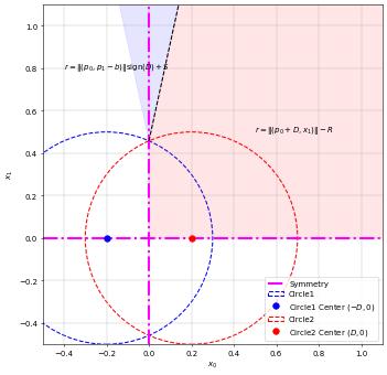
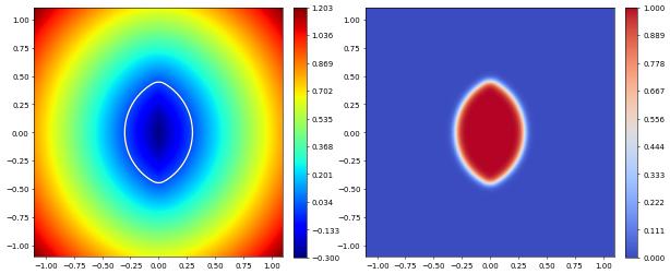
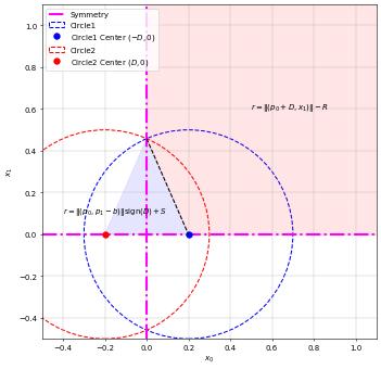
This shape is the same as two combined balls. Denoting, \(p = (|x_0|, |x_1|)^T\), and \(b = \sqrt{(R+S)^2 - D^2}\).

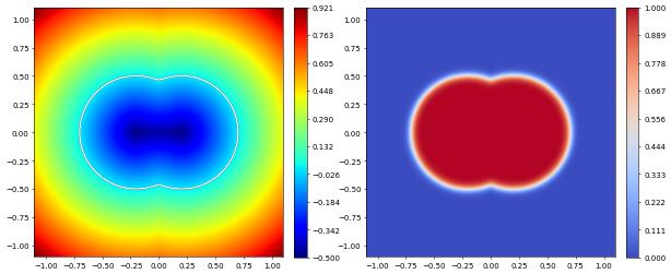
\[\begin{split}r(x) = \begin{cases} \| (p_0, p_1 - b) \| \text{sign}(D) + S & \text{if } (p_0 - b) D > p_1 b \\ \| (p_0 + D, x_1) \| - R & \text{otherwise} \end{cases}\end{split}\]

where \(R\) is the radius of the balls, \(D\) is the distance from origin (\(D > 0\) is intersection, \(D<0\) is union), and \(S\) is the smoothing factor.

Vesica, distance \(D > 0\)

[14]:

vesicaFigure()

[15]:

vesica1 = Vesica(radius=0.5, distance=0.2, smooth_radius=-0.1, epsilon=0.1)
plotSDF(vesica1)

Vesica, distance \(D < 0\)

[17]:

vesicaFigure()

[18]:

vesica2 = Vesica(radius=0.5, distance=-0.2, smooth_radius=0.1, epsilon=0.1)
plotSDF(vesica2)

Operations

[19]:

from ddfem.geometry import (
    Intersection,
    Invert,
    Round,
    Rotate,
    Scale,
    Subtraction,
    Translate,
    Union,
    Xor,
)

Binary Operations

We can combine two sign distance functions, \(r_1\) and \(r_2\), using the following operations:

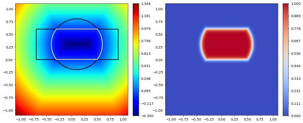
Intersection

\[r(x) = \max(r_1(x), r_2(x))\]

[20]:

plotSDF(box & circle)  # Intersection(box, circle)

Union

\[r(x) = \min(r_1(x), r_2(x))\]

[21]:

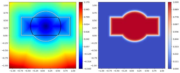
plotSDF(box | circle)  # Union(box, circle)

Subtraction

\[r(x) = \max(r_1(x), -r_2(x))\]

[22]:

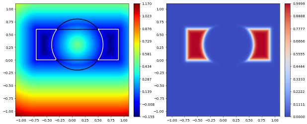
plotSDF(box - circle)  # Subtraction(box, circle)

Xor

\[r(x) = \max \left( \min( r_1(x), r_2(x) ), -\max( r_1(x), r_2(x) ) \right)\]

[23]:

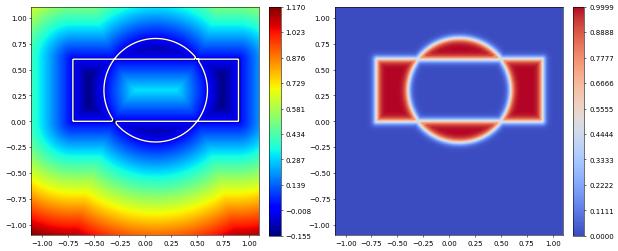
plotSDF(box ^ circle)  # Xor(box, circle)

It is important to acknowledge that the union, subtraction, and intersection operations do not produce a perfect SDF. However, as the width on the interfacial region is approximately \(2\epsilon\), the impact of the imperfect SDF on \(\phi\) is negligible.

Unary Operations

We can also modify individual SDFs, with the following operators:

Invert

\[r(x) = - r_1(x)\]

[24]:

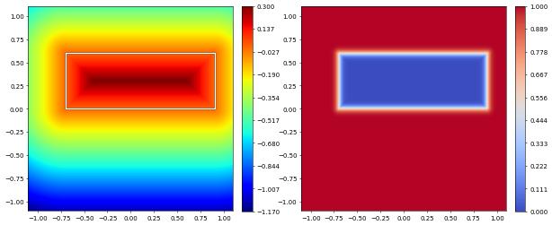
plotSDF(box.invert())  # Invert(box)

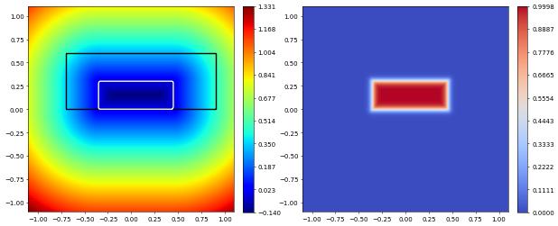
Scale

\[r(x) = s r_1(x / s)\]

where \(s > 0\) is the scaling factor.

[25]:

plotSDF(0.5 * box)  # Scale(box, 0.5)

Rotate

\[\begin{split}r(x) = r_1 \left( \begin{pmatrix} \cos(\theta) & \sin(\theta) \\ -\sin(\theta) & \cos(\theta) \end{pmatrix} x \right)\end{split}\]

[26]:

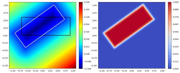
plotSDF(box.rotate(0.2 * pi))  # Rotate(box, 0.2*pi)

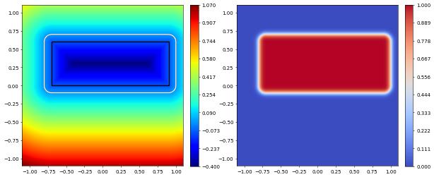
Round

\[r(x) = r_1(x) - s\]

where \(s\) is the scale factor for rounding distance.

[27]:

plotSDF(box.round(0.1))  # Round(box, 0.1)

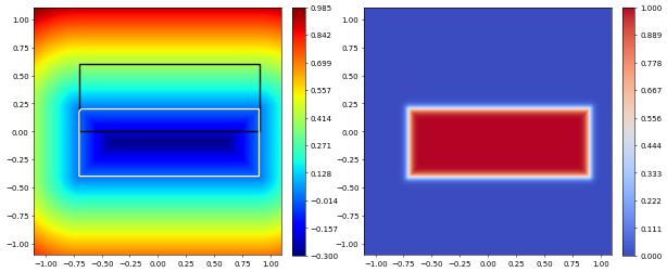
Translation

\[r(x) = r_1( x - v)\]

where \(v\) is the vector to translate by.

[28]:

plotSDF(box.translate(as_vector([0, -0.4])))  # Translate(box, as_vector([0, -0.4]))

3D examples

Most SDFs implemented will only compute using \(x_0\) and \(,x_1\). If Ball is given a center origin of a longer length, it will create that dimension’s of a ball.

[29]:

gv = dune.grid.structuredGrid([-1, -1, -1], [1, 1, 1], [50, 50, 50])
x = SpatialCoordinate(dune.ufl.cell(3))

sphere = Ball(radius=0.5, center=(0.1, 0.3, 0.1), epsilon=0.1)
# plotSDF(sphere) # can't currently inline plot 3d

We also have operators to extrude and revolve the existing 2D SDFs into 3D SDFs.

[30]:

from ddfem.geometry import Extrusion, Revolution

Extrusion

Denoting, \(d = r_1\left((x_0, x_1)^T\right)\), \(w = x_2 - L\). We have the signed distance function for the extruded SDF,

\[r(x) = \min( \max(d, w), 0 ) + \| (\max(d, 0), \max(w, 0))^T \|\]

where \(L\) is the extrusion length.

[31]:

from ddfem.geometry import Extrusion

cylinder = circle.extrude(length=1)  # Extrusion(circle, 1)

Revolve

To revolve around the \(x\)-axis, we have the signed distance functions,

\[r(x) = r_1\left( (x_0, \| (x_1, x_2) \| - s)^T \right)\]

To revolve around the \(y\)-axis, we have the signed distance functions,

\[r(x) = r_1\left( (\| (x_0, x_2) \| - s, x_0)^T \right)\]

where \(s\) is an offset from the axis.

[32]:

from ddfem.geometry import Revolution

torus = circle.revolve(0.6, "x")  # Revolution(circle, 0.6, "x" )

This page was generated from the notebook geometry_nb.ipynb and is part of the tutorial for the ddfem package using the dune-fem python bindings