from matplotlib import pyplot as plt

This notebook combines and extends code snippets from our paper […].

We start with some Dune specific includes that should be not too dificult to replace with code from other packages using UFL:

Dune specific code

from dune.fem.function import gridFunction
from dune.ufl import DirichletBC, Space

from ddfem import solve

Note the DDFEM package assumes the use of vector valued spaces. So will used a dummy vector valued space from \(\mathbb{R}^2\to \mathbb{R}^1\).

In the above solve function this is replace with a Lagrange space which is also vector valued (with vector length one):

space = Space(2, dimRange=1)

An Advection-Diffusion problem

Consider the problem

\[- \nabla \cdot D \nabla u + \nabla \cdot (b u) + c u = f\]

with Dirchlet boundary conditions \(u=g\) on the unit circle \(\Omega=B_1(0)\).

We use the coefficients, \(D(x) = 0.1 - 0.05 x \cdot x\), \(b(x) = 3 x^\perp\), \(c(x) \equiv 0.01\), \(f(x) = 0.1 (1 - x \cdot x)\), \(g(x) = \sin{(\pi x_0)}\sin{(\pi x_1)}\).

To define the model we use ufl. Remember to use ufl.as_vector to ensure all terms are vector valued.

Currently our transformers assume that the models are time dependent so, we define the methods to include a dummy time variable:

import ufl

D = lambda x: 0.1 - 0.05 * ufl.dot(x, x)
b = lambda x: 3 * ufl.as_vector([x[1], -x[0]])
c = lambda x: 0.01
f = lambda x: 0.1 * ufl.as_vector([1 - ufl.dot(x, x)])
g = lambda x: ufl.as_vector([ufl.sin(ufl.pi * x[0]) * ufl.sin(ufl.pi * x[1])])


class FittedModel:
    def S_i(t, x, U, DU):
        return f(x) - c(x) * U

    def F_c(t, x, U):
        return ufl.outer(U, b(x))

    def F_v(t, x, U, DU):
        return D(x) * DU

    boundary = {(1,): lambda t, x: g(x)}

The following functions convert a given Model class into a ufl form including the Dirchley boundary conditions:

def model2ufl(Model, space, DirichletBC):
    u, v = ufl.TrialFunction(space), ufl.TestFunction(space)
    x = ufl.SpatialCoordinate(space)
    t = 0

    si = -Model.S_i(t, x, u, ufl.grad(u))
    fc = -Model.F_c(t, x, u)
    fv = Model.F_v(t, x, u, ufl.grad(u))
    form = ufl.inner(fv + fc, ufl.grad(v)) + ufl.inner(si, v)
    dbcs = [
        DirichletBC(space, value(t, x), region)
        for regions, value in Model.boundary.items()
        for region in regions
    ]
    return [form * ufl.dx == 0, *dbcs]

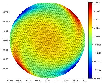
Let’s test this on a fitted grid constructed using gmsh:

import pygmsh

with pygmsh.occ.Geometry() as geom:
    geom.characteristic_length_max = 0.05
    geom.characteristic_length_min = 0.05
    disks = geom.add_disk([0, 0, 0], 1)
    mesh = geom.generate_mesh()
    points, cells = mesh.points, mesh.cells_dict
    domain = {
        "vertices": points[:, :2].astype(float),
        "simplices": cells["triangle"].astype(int),
    }

uh = solve(model2ufl(FittedModel, space, DirichletBC), domain)

fig = plt.figure(figsize=[6, 6])
uh.plot(figure=fig)

A diffuse domain approximation by hand

We will now use a simple diffuse domain approximation to solve the above problem on a larger square domain.

This requires an approximation to the domain’s characteristic function, \(\chi\), by a phase field, \(\phi\). A common choice is

\[\phi(x) = \frac{1}{2} \left(1 - \tanh\left(\frac{3 r(x)}{\varepsilon}\right)\right)\]

where \(r(x)\) denotes the signed distance function (SDF) for the domain. For this domain it is easy to define the domain SDF as the following:

def sdf(x):
    return ufl.sqrt(ufl.dot(x, x)) - 1

This phase field has the interfacial region width approximately \(2\epsilon\). To ensure sufficient resolution of this region and to reduce the impact on the solution, we use \(\varepsilon = 4.5 h\) where the \(h\) is the grid spacing:

domain = [[-1.25, -1.25], [1.25, 1.25], [50, 50]]
h = 2.5 / 50
epsilon = 4.5 * h
print(f"h={h}, epsilon={epsilon}")


def phi(x):
    return 0.5 * (1 - ufl.tanh(3 * sdf(x) / epsilon))

h=0.05, epsilon=0.225

In addition, it is convient to define some projection operators for reformulating the problem into the larger domain:

def chi(x):
    return ufl.conditional(sdf(x) <= 0, 1, 0)


def projection(x):
    return -ufl.grad(sdf(x)) * sdf(x)


def boundary_projection(x):
    return x + projection(x)


def external_projection(x):
    return x + (1 - chi(x)) * projection(x)


bp = boundary_projection
ep = external_projection

The simplest diffuse domain method is given by the DDM1 approach:

class ModelDDM1:
    def S_i(t, x, U, DU):
        outFactor = 3 + 0.1  # weighting chosen for this problem

        source = phi(x) * (f(ep(x)) - c(ep(x)) * U)
        bc = -outFactor * (U - g(bp(x))) * (1 - phi(x)) / (epsilon**3)

        return source + bc

    def F_c(t, x, U):
        return phi(x) * ufl.outer(U, b(ep(x)))

    def F_v(t, x, U, DU):
        return phi(x) * D(ep(x)) * DU

    boundary = {range(1, 5): lambda t, x: g(bp(x))}

For a sufficiently extended domain, the new extended domain boundary conditions will not significantly impact the solution. Above we can use chosen to extend g for a natural choice, which provides minior accuracy benefit.

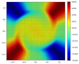
Now we can solve the problem on a square domain:

uh = solve(model2ufl(ModelDDM1, space, DirichletBC), domain)
fig = plt.figure(figsize=[6, 6])
uh.plot(figure=fig)

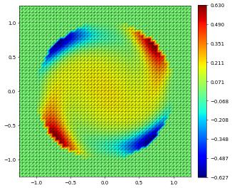
To compare with the fitted version we can plot the solution multiplied with the characteristic function:

fig = plt.figure(figsize=[6, 6])
x = ufl.SpatialCoordinate(space)
gridFunction(uh * chi(x)).plot(figure=fig)

Using this package

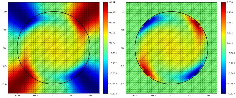
Instead of defining everything by hand let us use this package. The only change required to the Model is changing the boundary attribute to use the BndValue tag class. This is for ddfem.model2ufl to easily idenfify the different boundary types.

In addition, we need to define the factor to use for the penalisation on the outside domain. (See above, we haveoutFactor.) The penalisation term can be added to either the S_i or S_e method by setting the penalisation terms outFactor_i and outFactor_e respectively.

import ddfem

ball = ddfem.geometry.Ball(radius=1, name="full", epsilon=epsilon)


class Model(FittedModel):
    boundary = {"full": ddfem.boundary.BndValue(FittedModel.boundary[(1,)])}
    outFactor_i = 0.1
    outFactor_e = 3


ModelDDM1 = ddfem.transformers.DDM1(Model, ball)

uh = solve(ddfem.model2ufl(ModelDDM1, space, DirichletBC=DirichletBC), domain)
ddfem.plotSolution(ball, uh, figsize=[16, 8])

Flux boundary

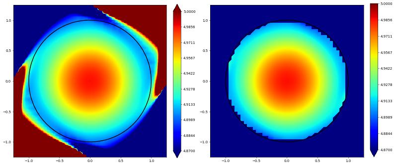
Switching from Dirichlet to flux boundary conditions is easily achieved. Since we have both a convective and diffusive flux, we need to provide boundary conditions for both type of fluxes in a list using BndFlux_v and BndFlux_c:

gf = lambda x: ufl.as_vector([ufl.tanh(10 * x[0] * x[1]) / 2])


class FluxModel(Model):
    boundary = {
        "full": [
            ddfem.boundary.BndFlux_v(lambda t, x, U, DU, n: gf(x)),
            ddfem.boundary.BndFlux_c(lambda t, x, U, n: gf(x)),
        ]
    }


ModelDDM1 = ddfem.transformers.DDM1(FluxModel, ball)

uhFlux = solve(ddfem.model2ufl(ModelDDM1, space, DirichletBC=DirichletBC), domain)
ddfem.plotSolution(ball, uhFlux, figsize=[16, 8], clim=[4.87, 5], gridLines=None)

A more complex domain

It is not a trivial task to directly provide a SDF for the geometry of a complex domain. The ddfem.geometry subpackage provides an interface to build the domain using simple shapes via constructive solid geometry.

You can easily define your own primitive shapes by extending the ddfem.geometry.SDF base class and implementing the SDF.sdf method.

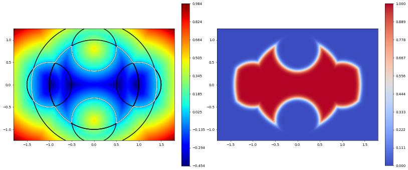
Here we have an example of combining five balls together. Each SDF contains a tree of the composing SDFs, which can be referenced to by setting an optional name.

from ddfem.geometry import Ball
from ddfem.geometry.domain_dune import DomainDune as Domain

domain = [[-1.8, -1.25], [1.8, 1.25], [135, 90]]
h = max(2.5 / 80, 3.6 / 120)
epsilon = 4.5 * h
print(f"h={h}, epsilon={epsilon}")


sdfs = [
    Ball(radius=1, center=(0, 0), name="Center"),
    Ball(radius=0.5, center=(0, 0.8), name="TopCut"),
    Ball(radius=0.5, center=(0, -0.8), name="BotCut"),
    Ball(radius=0.5, center=(1, 0), name="RightAdd"),
    Ball(radius=0.5, center=(-1, 0), name="LeftAdd"),
    Ball(radius=1.4, center=(0, 0), name="Cutoff"),
]

bulk = sdfs[0] - sdfs[1] - sdfs[2] | sdfs[3] | sdfs[4]
bulk.name = "bulk"
fiveBallSDF = bulk & sdfs[5]
fiveBallSDF.name = "full"
fiveBallSDF.epsilon = epsilon


omega = Domain(fiveBallSDF, domain)
gridView = omega.gridView

h=0.03125, epsilon=0.140625

ddfem.plot.plotSdfTree(fiveBallSDF, gridView, figsize=[16, 8], gridLines=None)

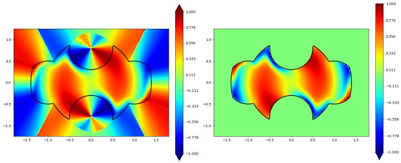
Solving the previous Dirchlet problem on this new domain gives:

ModelDDM1 = ddfem.transformers.DDM1(Model, omega)
uhDDM1 = solve(ddfem.model2ufl(ModelDDM1, space, DirichletBC=DirichletBC), gridView)
ddfem.plotSolution(omega, uhDDM1, figsize=[16, 8], clim=[-1, 1], gridLines=None)

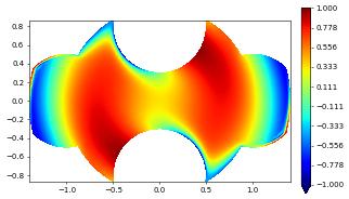
Let’s compare to a fitted mesh.

with pygmsh.occ.Geometry() as geom:
    geom.characteristic_length_max = h / ufl.sqrt(2)
    geom.characteristic_length_min = h / ufl.sqrt(2)
    disks = [geom.add_disk([c.center[0], c.center[1], 0.0], c.radius) for c in sdfs]

    disk_removed1 = geom.boolean_difference(disks[0], disks[1])
    disk_removed2 = geom.boolean_difference(disk_removed1, disks[2])

    disk_add = geom.boolean_union([disk_removed2, disks[3], disks[4]])
    shape = geom.boolean_intersection([disk_add, disks[5]])

    mesh = geom.generate_mesh()
    points, cells = mesh.points, mesh.cells_dict
    fittedDomain = {
        "vertices": points[:, :2].astype(float),
        "simplices": cells["triangle"].astype(int),
    }


uhFitted = solve(model2ufl(FittedModel, space, DirichletBC), fittedDomain)
fig = plt.figure(figsize=[6, 4])
uhFitted.plot(gridLines=None, clim=[-1, 1], figure=fig)

Info    : Cannot bind existing OpenCASCADE surface 1 to second tag 4
Info    : Could not preserve tag of 2D object 4 (->1)
Info    : Cannot bind existing OpenCASCADE surface 1 to second tag 5
Info    : Could not preserve tag of 2D object 5 (->1)
Info    : Cannot bind existing OpenCASCADE surface 1 to second tag 6
Info    : Could not preserve tag of 2D object 6 (->1)

print(f"Unfitted grid size is {gridView.size(2)}")
print(f"fitted grid size is {uhFitted.gridView.size(2)}")

Unfitted grid size is 12376
fitted grid size is 7236

Transformers

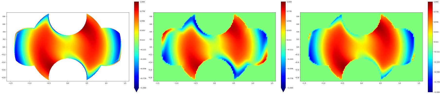
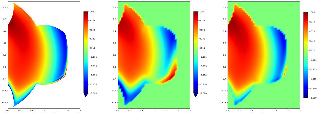
Several transfomers have been implemented. Each have benefits and tradeoffs with respect to accuracy and convergence. Here we will compare the DDM1 method we’ve seen so far to the Mix0DDM method. This approach was designed from the focus on Dirichlet boundary conditions, and is good at approximating gradients due from its design.

ModelMix0 = ddfem.transformers.Mix0DDM(Model, omega)
uhMix0 = solve(ddfem.model2ufl(ModelMix0, space, DirichletBC=DirichletBC), gridView)

So we compare all all three approaches. We see that bulk is similar but note the differences close to the boundaries.

fig, axs = plt.subplots(1, 3, figsize=[36, 8])
plotArgs = {
    "gridLines": None,
    "clim": [-1, 1],
    "xlim": [-1.6, 1.6],
    "ylim": [-0.9, 0.9],
    "linewidth": 0.4,
}

gridFunction(uhFitted).plot(**plotArgs, figure=(fig, axs[0]))
gridFunction(omega.chi(x) * uhDDM1).plot(**plotArgs, figure=(fig, axs[1]))
gridFunction(omega.chi(x) * uhMix0).plot(**plotArgs, figure=(fig, axs[2]))

fig, axs = plt.subplots(1, 3, figsize=[22, 8])
plotArgsZoom = plotArgs.copy()
plotArgsZoom["xlim"] = [0.4, 1.6]

gridFunction(uhFitted).plot(**plotArgsZoom, figure=(fig, axs[0]))
gridFunction(omega.chi(x) * uhDDM1).plot(**plotArgsZoom, figure=(fig, axs[1]))
gridFunction(omega.chi(x) * uhMix0).plot(**plotArgsZoom, figure=(fig, axs[2]))

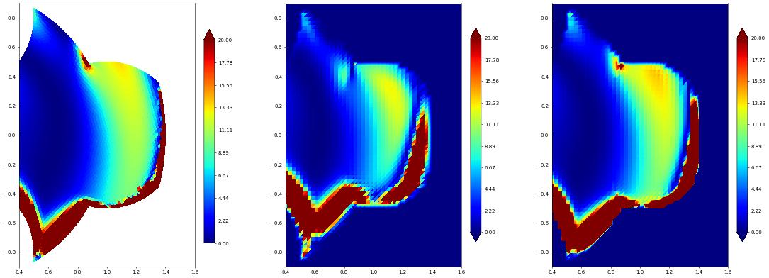
Each transformer has a sigma method defined to return the gradient. By default this is equal to the gradient, however, for example Mix0DDM also incorporates the boundary data.

absGrad = lambda du: ufl.inner(du, du)
fig, axs = plt.subplots(1, 3, figsize=[36, 8])
plotArgs["clim"] = [0, 20]

DuhFitted = ufl.grad(uhFitted)
DuhDDM1 = ModelDDM1.sigma(0, x, uhDDM1)
DuhMix0 = ModelMix0.sigma(0, x, uhMix0)

gridFunction(absGrad(DuhFitted)).plot(**plotArgs, figure=(fig, axs[0]))
gridFunction(omega.chi(x) * absGrad(DuhDDM1)).plot(**plotArgs, figure=(fig, axs[1]))
gridFunction(omega.chi(x) * absGrad(DuhMix0)).plot(**plotArgs, figure=(fig, axs[2]))

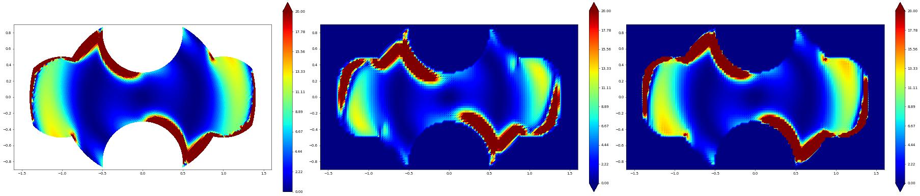
Again, zooming in we can see the differences more clearly.

fig, axs = plt.subplots(1, 3, figsize=[22, 8])
plotArgsZoom["clim"] = [0, 20]

gridFunction(absGrad(DuhFitted)).plot(**plotArgsZoom, figure=(fig, axs[0]))
gridFunction(omega.chi(x) * absGrad(DuhDDM1)).plot(**plotArgsZoom, figure=(fig, axs[1]))
gridFunction(omega.chi(x) * absGrad(DuhMix0)).plot(**plotArgsZoom, figure=(fig, axs[2]))

Special features using Dune-Fem

So far we have only used Dune-Fem for plotting and for solving the PDEs, and other packages could have been used.

Filtering

A benefit of using Dune-Fem for this diffuse domains, is the filtered grid view. This allows us to keep defining a large simple mesh, then remove points far away from the boundary to only compute on a subset of the mesh.

omega = Domain(fiveBallSDF, domain, filterTolerance=0.2)
gridView = omega.gridView

print(f"filtered grid size is {gridView.size(2)}.")
ddfem.plot.plotSdfTree(fiveBallSDF, gridView, figsize=[16, 8], gridLines=None)

filtered grid size is 7052.

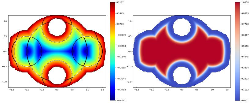
Note, due to the imperfect nature of combining SDFs in this way, the filtering may include unexpected regions further away. See Geometry Operators. For example, in this domain we get an extra loop at the top and bottom of the cut away balls.

Adaptivity

Dune-Fem also provides a straight forward way to locally adapt the mesh from a given function. Therefore, we can use the phase field with phi * (1 - phi) to easily mark the edge for refinement.

domain = [[-1.8, -1.25], [1.8, 1.25], [54, 36]]
omegaAdapt = Domain(fiveBallSDF, domain, filterTolerance=0.2, factor=0.5, refinements=4)
gridViewAdapt = omegaAdapt.gridView

print(f"Adaptive and Filtered grid size is {gridViewAdapt.size(2)}")
print(f"Fitted grid size is {uhFitted.gridView.size(2)}")

Adaptive and Filtered grid size is 3347
Fitted grid size is 7236

This combination of adaptivity and filtering has given use a mesh with fewer points than the uniform fitted mesh.

So now lets compare the different meshes.

ModelMix0adapt = ddfem.transformers.Mix0DDM(Model, omegaAdapt)
uhMix0adapt = solve(ddfem.model2ufl(ModelMix0adapt, space, DirichletBC=DirichletBC), gridViewAdapt)

fig, axs = plt.subplots(1, 3, figsize=[22, 8])
plotArgsZoom["gridLines"] = "black"
plotArgsZoom["clim"] = [-1, 1]

gridFunction(uhFitted).plot(**plotArgsZoom, figure=(fig, axs[0]))
gridFunction(omega.chi(x) * uhMix0).plot(**plotArgsZoom, figure=(fig, axs[1]))
gridFunction(omega.chi(x) * uhMix0adapt).plot(**plotArgsZoom, figure=(fig, axs[2]))

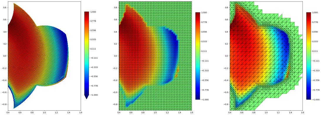
We can clearly see how this improves the solution computed close to the boundary.

fig, axs = plt.subplots(1, 3, figsize=[22, 8])
plotArgsZoom["clim"] = [0, 20]

DuhMix0adapt = ModelMix0adapt.sigma(0, x, uhMix0adapt)
gridFunction(absGrad(DuhFitted)).plot(**plotArgsZoom, figure=(fig, axs[0]))
gridFunction(omega.chi(x) * absGrad(DuhMix0)).plot(**plotArgsZoom, figure=(fig, axs[1]))
gridFunction(omega.chi(x) * absGrad(DuhMix0adapt)).plot(**plotArgsZoom, figure=(fig, axs[2]))

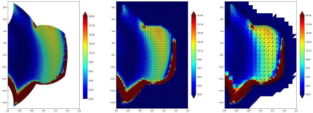
This page was generated from the notebook intro_nb.ipynb and is part of the tutorial for the ddfem package using the dune-fem python bindings